

Reduction of on-off observations with BoA
The doOO function
On-off scans (a.k.a. woo, or photometry mode) observed with LABOCA or SABOCA can be processed using the BoA function doOO(). Here is the header of this function:
def doOO(scanlist=[],tau=0.3,subscans=[],weak=1,filename='',update=0,source='',clip=2.0):
    """
    NAM: doOO (function)
    DES: this function processes a list of ON-OFF scans
    INP: (i list) scanlist : list of scan numbers
         (float) tau       : zenith opacity (same is applied to all scans)
         (i list) subscans : optional list of subscans to consider
                            (default = all subscans)
         (bool) weak       : processing optimised for weak sources? (def.=1)
         (str) filename    : optional name of a text file, where results are
                             written out, AND from which previous results are
                             read in if the argument 'update' is set to 1
         (bool) update     : if set, read previous results from file 'filename'
         (str) source      : name of the target (used in plot titles)
         (float) clip      : when reading previous results (i.e. when update=1),
                             measurements at more than clip*sigma from the mean
                             value are discarded
    """
More details about each argument of this function are given below.
| Argument | Explanation |
|---|---|
| scanlist | List of scan numbers to be processed, e.g. [12213,12215], range(9876,9889). Also to process a single scan, a list is required, like [12321]. |
| tau | Zenith opacity. This is a single value, applied to all the data to be processed. Default value is 0.3. WARNING: this function does NOT use the opacity derived from PWV if no value is given for tau. |
| subscans | Optionally, provides a list of subscans to be processed within the scan(s); for example: subscans=[1,2,5,6]. When used in combination with a list of scans, for each scan only the subscans given in this list will be processed. |
| weak | Boolean flag to specify if the reduction should be optimized for weak or strong source. A source can be considered weak when its flux density is less than 100 mJy. For a source with, for example, a flux density of 250 mJy, using weak=1 reduces the flux by 15%, because real data are flagged during the reduction, due to more iterations of correlated noise removal. |
| filename | A character string specifying the name of a file used, both, for input and output. If no filename is given, the results are only written on the screen, but not saved. If a filename is given, the results for each nodding cycle (i.e. two subscans) are written in this text file. In addition, if the argument update is True, then previous results written in that file are read in and included in the computation of the final result. Warning: with arguement update=0 (see below), if a file with that name already exists, it will be overwritten. |
| update | Flag to specify that the results previously written in the file with name 'filename' have to be included in the final result. New results will be appended at the end of this file. |
| source | A character string used only in the caption of the plots. |
| clip | When reading previous results (i.e. when update=1), the mean value and standard deviation (sigma) are computed. Then, measurements outside the range mean ± clip*sigma are discarded and not used in the final result. |
Cookbook
Here are the different steps required for a typical reduction of a series of on-off scans on a given target. This involves: calibration of the data, starting reduction of the first scan(s), adding more data, and computing the final result.Calibration
First thing to do is to determine zenith opacity for all the data to be processed. The easiest case is to assign one opacity value for each scan, or group of scans. But if the opacity is changing rapidly within a scan, it is also possible to process individual nodding cycles (= two subscans) with different opacity values.To determine zenith opacities, the user can reduce the skydips included in his/her dataset, or refer to the LABOCA sky opacity query page. If calibrations performed close in time with the woo observations show that an extra calibration correction factor has to be applied, this has to be done mannually, i.e. the results (flux and associated errors) have to be scaled directly in the output text file. For example, if only 90% of the expected flux is measured on calibrators, the woo results have to be divided by 0.90 in order to correct the calibration.
First scan on a source
When reducing the first set of data on a given source (this can be a single scan, or a list of scans, all observed with the same zenith opacity), one has to call the doOO function with the argument update=0, and give a file name where the results for each individual measurement are written in text format.doOO(scanlist=[....],tau=x.x,weak=0/1,filename='YOUR FILE NAME',update=0)For example:
doOO(scanlist=[12215],tau=0.24,weak=1,filename='J123456-oo.dat',update=0)
For each individual measurement, i.e. each nodding cycle (= one pair of subscans), one line is written in the output file, with the following format:
  flux       err_flux  NEFD   time   off_flux    err_off
  0.026126   0.020652  57.49  20.24  -0.001389   0.025814
where the different columns have the following meaning:
- flux: result of ON - OFF measurement, in Jy
- err_flux: associated statistical uncertainty
- NEFD: instrumental Noise Equivalent Flux Density, in mJy sqrt(s)
- time: ON-source time (in seconds)
- off_flux: average of OFF-bolo fluxes
- err_off: associated statistical uncertainty
At the end of the reduction, the function displays the "final result" on the screen. This output looks like the following example:
###################################################
Final result =  32.67 +/-   8.80 [+/-  14.99] mJy/b
Average OFF bolo =  -1.72 +/-  10.5 mJy/b
Effective NEFD:   65.6 mJy sqrt(s)
12215   32.67   8.80   0.01   -1.72  10.53   65.6
###################################################
The most important numbers are written in the first line:
Final result = FLUX +/- sigma_1 [+/- sigma_2] mJy/b- FLUX is the mean value (weighted average) of all ON - OFF measurements,
- sigma_1 is the theoretical uncertainty on FLUX, computed assuming that all measurements are independent. It is computed as sqrt[1/sum(1/σ2)], where σ is the statistical uncertainty associated to each measurement (i.e. err_flux, which is written in the 2nd column of the output file),
- sigma_2 is the actual statistical uncertainty, measured on the data. This is computed as the standard deviation of all measurements, divided by the square root of the number of measurements.
Important note: sigma_1 almost always underestimates the true uncertainty, and should not be used to estimate the significance of a detection, or to compute an upper limit. The uncertainty to be quoted in the final result is given by sigma_2.
In addition, the function produces a plot, similar to the following one:
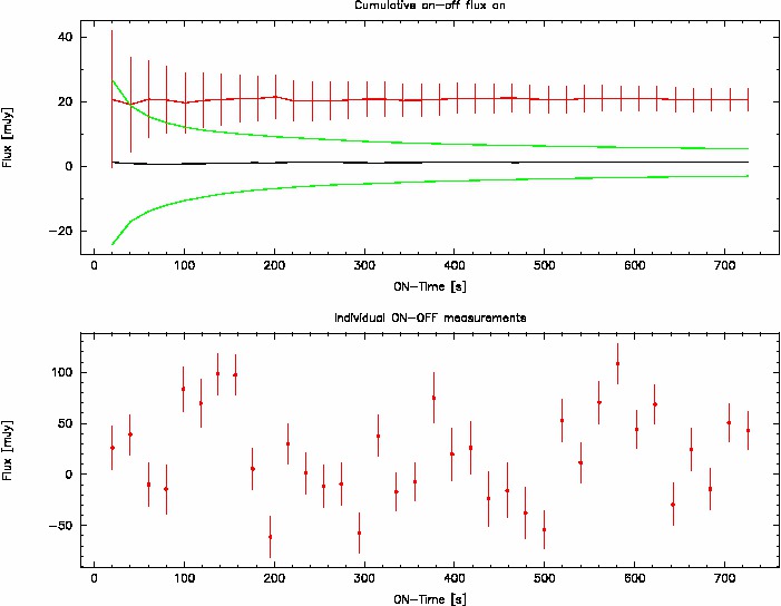
This plot provides the following information:
- Top panel: cumulative plots.
- The black line shows the evolution of the mean value of all OFF-bolometers when adding more and more data.
- The two green lines show the evolution of off_flux ± err_off.
- The red line shows the evolution of the ON - OFF measurement, with error bars that correspond to the theoretical uncertainty.
- Bottom panel:Individual measurements with associated error bars are shown as a function of cumulated ON-source time. It follows the sequence along which the data have been reduced and written into the text file.
Note that there is no one-to-one correspondance between the two plots, because in order to produce the cumulative average plot, the individual measurements are shuffled many times, and then the average of all this shuffling is computed. For example, the 3rd point corresponds to the average of many realizations of choosing 3 measurements among all the measurements available.
Adding new data
When more data become available, to include them in the reduction requires to call the function with argument update=1, and to give the name of the file that was previously created. For example:doOO(scanlist=[12217],tau=0.23,weak=1,filename='J123456-oo.dat',update=1)The new results are then appended at the end of the file. The outputs on the screen (text and plots) have the same meaning as previously.
![]() WARNING: You should give only scan numbers that have not already been
processed and written in the output file. Since the scan numbers are not
written in the file, the function cannot determine if some scans have
already been processed; thus, they would be reduced again and the
results would be appended in the file, and would then be used several
times to compute the final average.
WARNING: You should give only scan numbers that have not already been
processed and written in the output file. Since the scan numbers are not
written in the file, the function cannot determine if some scans have
already been processed; thus, they would be reduced again and the
results would be appended in the file, and would then be used several
times to compute the final average.
Computing the final result
Finally, when all the data have been processed, it can be a good idea to clip some outliers. To do this, one has to call the doOO function with an empty list as input scan list, and with update=1 and the name of the file where the results have been written. In addition, one can specify the number of sigma (κ) that defines the range where to start clipping: values below mean - κσ or above mean + κσ are discarded, and not included in the computation of the final result. The default value for κ is 2.0.doOO([],filename='J123456-oo.dat',update=1) # default: clip=2.0 doOO([],filename='J123456-oo.dat',update=1,clip=3.) # clip at 3-sigma